Unlocking The Power Of FEM: A Comprehensive Guide To The Finite Element Method
In the vast landscape of engineering and scientific inquiry, understanding and predicting the behavior of complex systems is paramount. From designing resilient bridges to simulating blood flow in arteries, engineers and scientists constantly seek robust tools to tackle intricate problems. This is precisely where the Finite Element Method (FEM) steps in, offering a powerful numerical approach to solve differential equations that govern these real-world phenomena. It's a cornerstone in modern computational mechanics, enabling breakthroughs across countless disciplines.
If you've ever wondered how engineers predict the stress on an airplane wing, the heat distribution in an engine, or the fluid dynamics around a car, chances are the Finite Element Method (FEM) played a crucial role. This detailed guide will demystify this complex yet indispensable technique, explaining its core principles, applications, and why it has become the dominant method for solving challenging problems in various fields. Prepare to dive into the world where mathematics meets engineering, transforming theoretical equations into practical insights.
Table of Contents
- What is the Finite Element Method (FEM)?
- The Evolution of FEM: A Glimpse into its History
- FEM vs. FEA: Understanding the Core Difference
- The Workflow of a Finite Element Analysis (FEA): A Step-by-Step Approach
- Delving Deeper: Partial Differential Equations (PDEs) in FEM
- Key Technical Concepts in Mastering FEM
- Typical Applications of the Finite Element Method Across Industries
- Why FEM Reigns Supreme: Advantages and Limitations
What is the Finite Element Method (FEM)?
The Finite Element Method (FEM) is a popular method for numerically solving differential equations arising in engineering and mathematical modeling. At its core, FEM is a powerful numerical technique that is used to obtain approximate solutions to problems that are governed by differential equations. These equations often describe physical phenomena that are too complex to solve analytically, meaning there's no neat, closed-form mathematical expression for their solutions.
In short, FEM is used to compute approximations of the real solutions to PDEs. Instead of trying to find a solution that applies to an entire continuous domain (like a whole bridge or a complete fluid flow), FEM breaks down this complex domain into a finite number of smaller, simpler pieces called "elements." These elements are interconnected at specific points called "nodes." Within each element, the unknown solution is approximated using simple functions, typically polynomials. By assembling the contributions from all these individual elements, the method constructs a system of algebraic equations that can then be solved to find the approximate solution over the entire domain.
Typical problem areas of interest include structural mechanics, heat transfer, fluid flow, electromagnetism, and acoustics. For instance, in structural mechanics, FEM is the dominant discretization technique, allowing engineers to predict how a structure will deform or fail under various loads. It transforms a continuous problem into a discrete one, making it amenable to computer calculations.
The Evolution of FEM: A Glimpse into its History
To truly appreciate the power of the Finite Element Method, it's insightful to understand its origins. What is the history of the finite element method? The roots of FEM can be traced back to the early 20th century, with methods like the Rayleigh-Ritz method and Galerkin method laying theoretical groundwork for approximating solutions to differential equations. However, the method as we know it today truly began to take shape in the 1940s and 1950s, primarily driven by the demands of the aerospace industry.
During World War II and the subsequent Cold War era, engineers faced unprecedented challenges in designing complex aircraft structures. Traditional analytical methods were insufficient for analyzing the intricate stress distributions in these new designs. In 1943, Richard Courant, a mathematician, used a method of piecewise polynomial interpolation over triangular subregions to solve torsion problems, which is often cited as a foundational precursor to FEM.
The term "Finite Element Method" itself was coined in 1960 by engineers at Boeing, Clough, and others, who were developing practical computational techniques for structural analysis. Their work, alongside contributions from researchers at UC Berkeley, MIT, and other institutions, solidified the method's practical application. The advent of digital computers in the 1950s and 60s was crucial, as FEM is inherently computationally intensive. Without the ability to perform vast numbers of calculations rapidly, the method would have remained largely theoretical.
From its initial focus on structural mechanics, FEM rapidly expanded its reach to other fields, demonstrating its versatility and robustness. Its continuous development, fueled by advancements in computer hardware and numerical algorithms, has made it an indispensable tool in virtually every engineering discipline today.
FEM vs. FEA: Understanding the Core Difference
It's common to hear the terms "FEM" and "FEA" used interchangeably, but there's a crucial distinction between them. While FEM is a mathematical technique, FEA is the process. Let's break this down:
- Finite Element Method (FEM): This refers specifically to the underlying mathematical and numerical formulation. It's the theoretical framework, the set of equations and algorithms that allow for the approximation of solutions to differential equations. It's the "how" – how the problem is discretized, how the equations for each element are derived, and how they are assembled into a global system.
- Finite Element Analysis (FEA): This is the practical application of the Finite Element Method. Finite Element Analysis (FEA) is the process of predicting an object’s behavior based on calculations made with the finite element method (FEM). FEA encompasses the entire workflow, from preparing the geometric model, defining material properties, applying loads and boundary conditions, running the FEM calculations using specialized software, and finally, interpreting and visualizing the results. It's the "what" – what engineers actually do to solve a specific problem using the FEM.
Think of it this way: FEM is the engine, and FEA is the car. You need the engine (FEM) to make the car (FEA) move, but the car itself is the complete system that takes you from point A to point B. An engineer performs an FEA using software that implements the FEM. Understanding this distinction is vital for anyone delving into computational simulations.
The Workflow of a Finite Element Analysis (FEA): A Step-by-Step Approach
If you haven’t been hiding under a stone, you've likely encountered the results of FEA in various products and designs around you. But how does a finite element analysis (FEA) workflow look like? The process typically involves several key stages:
- Preprocessing (Model Setup):
- Geometry Definition: The first step is to create or import the geometric model of the object or system to be analyzed. This could be a 2D sketch or a complex 3D CAD model.
- Material Properties: Define the physical properties of the materials involved, such as Young's modulus, Poisson's ratio, density, thermal conductivity, etc. These properties dictate how the material will respond to applied forces or temperatures.
- Meshing (Discretization): This is where the Finite Element Method truly begins to shine. The continuous geometry is divided into a finite number of discrete elements. The quality and density of this mesh significantly impact the accuracy and computational cost of the analysis.
- Boundary Conditions and Loads: Apply the conditions that simulate the real-world environment. Boundary conditions define how the model is constrained (e.g., fixed supports, roller supports). Loads represent the external forces, pressures, temperatures, or displacements acting on the system.
- Solving (Analysis):
- Once the model is fully defined, the FEA software takes over. It uses the underlying Finite Element Method to assemble the stiffness matrices (or equivalent for other physics) for each element, then combines them into a global system of equations.
- This large system of algebraic equations is then solved to determine the unknown primary variables at the nodes (e.g., displacements in structural analysis, temperatures in thermal analysis, pressures in fluid analysis).
- Postprocessing (Results Interpretation):
- The raw numerical results from the solver are often difficult to interpret directly. Postprocessing tools visualize these results.
- Engineers can view contour plots of stress, strain, displacement, temperature distribution, velocity fields, etc. They can also generate animations, create reports, and extract specific numerical values at critical points. This stage is crucial for validating the design, identifying potential failure points, and optimizing performance.
This systematic workflow allows engineers to virtually test and refine designs, reducing the need for costly physical prototypes and accelerating product development cycles.
Delving Deeper: Partial Differential Equations (PDEs) in FEM
At the heart of the Finite Element Method lies the concept of Partial Differential Equations (PDEs). What partial differential equations are in FEM? PDEs are mathematical equations that involve an unknown function of multiple independent variables and their partial derivatives. They are the language through which most physical laws are expressed.
Consider a few examples:
- Structural Mechanics: The equilibrium of a deformable body under load is governed by PDEs that relate stresses, strains, and displacements. For example, the Navier-Cauchy equations describe elastic deformation.
- Heat Transfer: The distribution of temperature in an object over time is described by the heat equation, a type of PDE.
- Fluid Dynamics: The movement of fluids is governed by the Navier-Stokes equations, a complex set of PDEs that account for momentum, mass, and energy conservation.
- Electromagnetism: Maxwell's equations, a set of four PDEs, describe the behavior of electric and magnetic fields.
The challenge is that for most real-world geometries and boundary conditions, these PDEs are incredibly difficult, if not impossible, to solve analytically. This is where FEM becomes indispensable. The Finite Element Method (FEM) is a numerical method for solving partial differential equations (PDE) that occur in problems of engineering and mathematical physics. Instead of solving the PDE directly over the entire domain, FEM transforms the PDE into a system of algebraic equations over discrete elements. This transformation allows computers to approximate the solution, providing valuable insights into the behavior of the system described by the PDEs.
For example, consider the model problem u''(x) = 1, for x in (0,1) with u(0) = u(1) = 0. This is a simple ordinary differential equation (a special case of a PDE). The exact solution is u(x) = x(1-x)/2. While this specific problem has an exact solution, more complex versions with irregular shapes or varying material properties would necessitate FEM to find an approximate solution of the form suitable for numerical computation.
Key Technical Concepts in Mastering FEM
To truly grasp the power of the Finite Element Method, it's essential to understand its core technical underpinnings. What are the most important technical points to learn in FEM? Here are some fundamental concepts:
Discretization and Meshing: The Foundation of FEM
The basic concept in the physical interpretation of the FEM is the subdivision of the mathematical domain. This process, known as discretization, involves breaking down a continuous problem domain into a finite number of smaller, simpler subdomains called "finite elements." These elements are typically simple geometric shapes like triangles, quadrilaterals (2D), tetrahedra, or hexahedra (3D).
The process of creating these elements is called meshing. The nodes are the points where elements connect and where the unknown variables (like displacement or temperature) are calculated. The quality of the mesh is paramount:
- Element Shape and Size: Irregularly shaped or overly distorted elements can lead to inaccurate results. Smaller elements generally provide higher accuracy but increase computational cost.
- Mesh Density: Denser meshes (more elements) are typically used in areas where the solution is expected to change rapidly (e.g., stress concentrations around a hole) to capture details accurately.
- Element Types: Different types of elements (e.g., linear, quadratic) offer varying levels of approximation capabilities. Higher-order elements can approximate complex variations within an element more accurately but are computationally more expensive.
Effective meshing is often considered an art form in FEA, requiring experience and judgment to balance accuracy with computational efficiency.
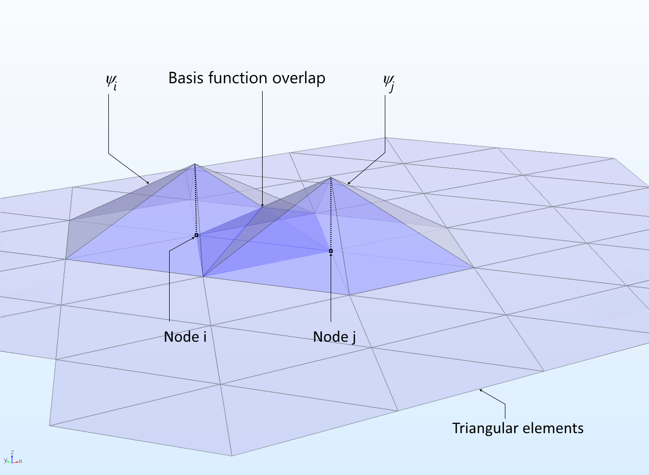
Basis Functions and Approximation: The Heart of FEM
Once the domain is discretized, FEM approximates the unknown solution within each element using simple functions, known as shape functions or basis functions. These functions are typically polynomials. For example, for a simple 1D element, a linear basis function might be used, meaning the solution varies linearly between the nodes of that element. For 2D elements, bilinear or quadratic functions are common.
The unknown solution (e.g., displacement) at any point within an element is expressed as a weighted sum of these basis functions, where the weights are the unknown nodal values. The goal is to find an approximate solution of the form that minimizes the error between the approximate solution and the true solution of the governing PDE. This is often achieved using methods like the Galerkin method, which ensures that the weighted average of the error over the domain is zero. This process transforms the continuous PDE into a set of discrete algebraic equations for each element.
Boundary Conditions and Load Application: Defining the Problem
For any physical problem, the behavior of the system is not only governed by its internal properties (material, geometry) but also by its interaction with the environment. This interaction is defined through boundary conditions and applied loads.
- Boundary Conditions: These specify how the system is constrained or fixed at its boundaries. Common types include:
- Dirichlet (Essential) Boundary Conditions: Specify the value of the primary unknown variable directly (e.g., fixed displacement at a point, prescribed temperature at a surface).
- Neumann (Natural) Boundary Conditions: Specify the derivative of the primary unknown variable or a flux (e.g., applied force, heat flux).
- Loads: These are the external influences acting on the system. They can be:
- Concentrated Loads: Applied at a single node (e.g., a point force).
- Distributed Loads: Applied over an area or volume (e.g., pressure, gravity).
- Thermal Loads: Changes in temperature causing expansion or contraction.
Accurately defining these conditions is critical, as they significantly influence the results of the Finite Element Analysis. Incorrect boundary conditions or loads will lead to erroneous predictions, regardless of how well the FEM is implemented.
Solving the System: From Equations to Solutions
Once the element equations are formulated and boundary conditions applied, they are assembled into a large global system of algebraic equations. For structural problems, this often takes the form of `[K]{U} = {F}`, where `[K]` is the global stiffness matrix, `{U}` is the vector of unknown nodal displacements, and `{F}` is the global force vector.
This system can contain thousands or even millions of equations, especially for complex 3D models. Specialized numerical solvers are employed to efficiently solve these large systems. These solvers can be direct (e.g., Gaussian elimination for smaller systems) or iterative (e.g., Conjugate Gradient method for very large systems). The solution of this global system yields the approximate values of the primary unknown variables at each node. From these nodal values, other quantities of interest (like stress, strain, heat flux, or velocity) can be calculated within each element during the post-processing phase. The efficiency and robustness of these solvers are crucial for the practical application of the Finite Element Method.
Typical Applications of the Finite Element Method Across Industries
The versatility of the Finite Element Method makes it applicable across an astonishing array of industries and problem types. Typical problem areas of interest include:
- Structural Mechanics: This is arguably where FEM first gained prominence and remains a dominant application. It's used to analyze stress, strain, deformation, vibration, and fatigue in structures ranging from bridges and buildings to aircraft components, automotive parts, and biomedical implants.
- Heat Transfer: FEM can simulate heat conduction, convection, and radiation to predict temperature distributions in electronic components, engine blocks, heat exchangers, and even in the human body.
- Fluid Dynamics (Computational Fluid Dynamics - CFD): While often using specialized methods, FEM is also employed in CFD to simulate fluid flow, pressure distribution, and aerodynamic forces around objects like cars, aircraft, and in pipelines.
- Electromagnetism: Used to analyze electric and magnetic fields, design antennas, motors, generators, and optimize electromagnetic shielding.
- Acoustics: Simulating sound propagation, noise reduction in vehicles, and the design of concert halls.
- Biomechanics and Biomedical Engineering: Analyzing stress on bones and implants, simulating blood flow, designing prosthetics, and understanding tissue mechanics.
- Geotechnical Engineering: Analyzing soil mechanics, foundation design, and stability of slopes.
- Manufacturing Processes: Simulating metal forming, welding, casting, and additive manufacturing to optimize processes and predict material behavior.
The ability of FEM to handle complex geometries, various material properties (linear, non-linear, isotropic, anisotropic), and diverse boundary conditions makes it an indispensable tool for research, design, and optimization in virtually every engineering discipline. It allows engineers to virtually test designs, identify potential flaws, and optimize performance long before physical prototypes are built, saving significant time and resources.
Why FEM Reigns Supreme: Advantages and Limitations
The widespread adoption of the Finite Element Method is not accidental; it stems from its significant advantages in tackling complex engineering problems. However, like any powerful tool, it also comes with certain limitations.
Advantages of FEM:
- Handles Complex Geometries: Unlike analytical methods that are often limited to simple shapes, FEM can analyze structures with highly intricate and irregular geometries.
- Versatility in Material Properties: It can accommodate a wide range of material behaviors, including isotropic, anisotropic, linear elastic, non-linear, plastic, and composite materials.
- Diverse Boundary Conditions and Loading: FEM can simulate various types of boundary conditions (fixed, roller, prescribed displacement) and complex loading scenarios (point loads, distributed loads, thermal loads, dynamic loads).
- Multi-Physics Capabilities: Modern FEM software can couple different physics phenomena, such as thermal-structural, fluid-structure interaction, or electro-thermal analyses, providing a more comprehensive understanding of system behavior.
- Cost and Time Savings: By allowing virtual prototyping and testing, FEM significantly reduces the need for expensive physical prototypes and extensive experimental testing, thereby accelerating the design cycle and reducing development costs.
- Detailed Insights: FEM provides detailed information about stress, strain, temperature, or flow fields throughout the entire domain, not just at a few discrete points, offering deep insights into the system's performance.
- Optimization: The results from FEM can be directly used in optimization algorithms to improve design performance, reduce material usage, or enhance safety.
Limitations of FEM:
- Computational Cost: For very large and complex models, especially those involving non-linear or transient analysis, the computational time and resources required can be substantial.
- Mesh Dependency: The accuracy of the solution is highly dependent on the quality and density of the mesh. Poor meshing can lead to inaccurate or misleading results.
- Expertise Required: Performing a reliable FEA requires significant expertise in both the underlying physics and the FEM itself. Incorrect model setup, boundary conditions, or interpretation of results can lead to critical errors.
- Approximation Nature: It provides approximate solutions, not exact ones. While often highly accurate for engineering purposes, it's crucial to understand the inherent approximation and potential sources of error.
- Software Complexity: High-end FEA software packages can be complex to learn and master, requiring extensive training.
Despite its limitations, the advantages of the Finite Element Method far outweigh its drawbacks for most engineering applications, solidifying its position as an indispensable tool in the modern world.
Conclusion
The Finite Element Method (FEM) stands as a monumental achievement in numerical analysis and computational engineering. As we've explored, it's not just a mathematical curiosity but a practical, indispensable tool that allows us to virtually test, analyze, and optimize designs across a myriad of industries. From its humble beginnings in aerospace to its current pervasive use in structural mechanics, heat transfer, fluid dynamics, and beyond, FEM has consistently proven its ability to provide approximate solutions to complex partial differential equations that would otherwise be intractable.
Understanding the distinction between FEM (the mathematical technique) and FEA (the applied process) is key, as is appreciating the detailed workflow involved in setting up, solving, and interpreting simulations. While the method demands careful application and a solid grasp of its underlying technical concepts—such as discretization, basis functions, and the critical role of boundary conditions—its benefits in terms of cost savings, accelerated development, and deep design insights are unparalleled. The power of FEM continues to drive innovation, enabling engineers to push the boundaries of what's possible.
Have you ever used FEM in your projects or studies? What challenges or successes have you experienced? Share your thoughts and insights in the comments below, or explore other articles on our site to deepen your understanding of computational engineering!
- Skylar Blue Sextape
- Montana Jordanleak
- Katie Sigmond Leaked Nude
- Sophie Rain Folder
- Scarlett Johansson Sexy Gif
![Finite Elemente Methode [FEM] - Einfach erklärt!](https://konstruktionsbude.de/wp-content/uploads/2023/01/FEM_Ergebnisse.png)
Finite Elemente Methode [FEM] - Einfach erklärt!
Detailed Explanation of the Finite Element Method (FEM)
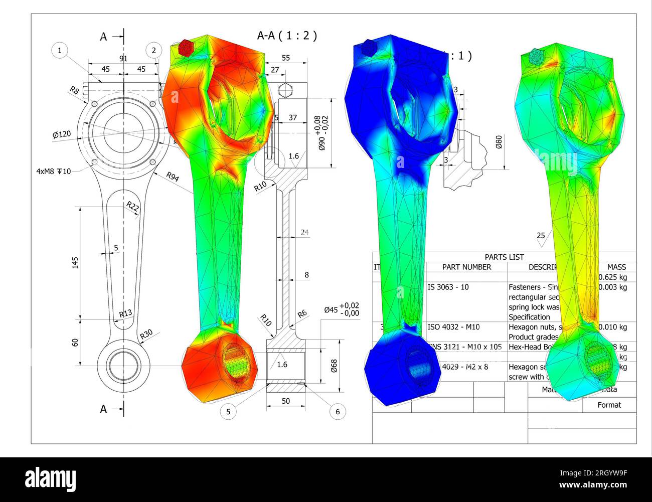
finite element method, FEM, analysis connecting rod crank for friction
